中文版:细菌怎样“数”分子
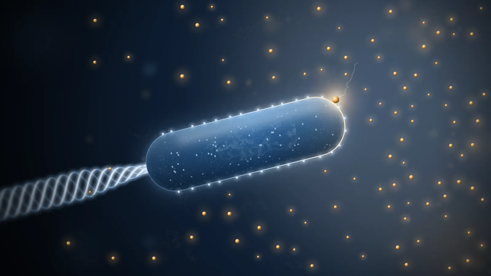
Imagine you are an E. coli.
You are about two micrometres long and pushed along by a few flagella behind you, at 30 micrometres a second, a dozen or so body lengths every second. You are hungry. There is sugar somewhere nearby, but you don’t know which way.
You have no eyes and no nose. What you have is a few thousand receptors scattered over your surface. Each can hold one sugar molecule at a time, for a moment, before letting it go. The only thing you can do is count: how many receptors are occupied now, and how many a little later. If the number is rising you are swimming towards more sugar, so keep going. If it is falling, stop, tumble, and try a new direction.
That sounds easy. Do the arithmetic and it turns out to be astonishingly hard.
Take a sugar concentration of 1 µM (one micromole per litre, a common concentration inside living things). A ball of water your size, one micrometre in radius, holds on average only about 2,500 sugar molecules. To tell that the concentration is 1% higher, you have to see a difference of 25 molecules out of 2,500. But those molecules never stop moving in and out, and their random fluctuation alone is about , twice the signal you are looking for.
Fig. 1 A ball one micrometre in radius holds on average 2,500 molecules at 1 µM (blue, solid) and 2,525 at a concentration 1% higher (ochre, dashed). The curves are the distributions of the number you get by averaging counts; the grey area is where the two can be mistaken for each other. Count once and you will say which concentration is higher only six times in ten, barely better than a guess. Drag the slider to see how many counts it takes to pull the curves apart. The time assumes one independent count per millisecond, a number explained in section 4.
So counting once is not enough; you have to count again and again and average. Which raises the questions:
- How long do you have to count to see a 1% difference?
- How many receptors do you need? Are a few thousand enough? How should they be arranged?
- If you swim faster, sweeping through the water like a net, can you catch more molecules?
In 1977 Howard Berg and Edward Purcell wrote a paper that works through these questions one by one. Berg was the first to watch E. coli swim in three dimensions, with a tracking microscope he built; Purcell was a physicist with a Nobel Prize for nuclear magnetic resonance. Their answers are unexpectedly elegant:
- Receptors covering just a thousandth of the cell surface catch half of everything the cell could possibly catch.
- Swimming, or stirring the water around you, hardly helps at all.
- The precision of a measurement depends on one number only: how many new molecules you have caught.
- Real E. coli operate close to the limit that physics allows.
Let’s derive these four results step by step. All you need to know is that diffusion means molecules wandering at random; any other mathematics is explained where it comes up. Every figure can be dragged and adjusted; they are computed live in your browser from the formulas.
Reading: H. C. Berg & E. M. Purcell, Physics of chemoreception, Biophys. J. 20, 193–219 (1977). Equation numbers follow the original.
1How many molecules can a cell swallow per second?
Start with the simplest possible version. Forget the receptors and treat the cell as a “black hole” of radius that swallows every molecule touching its surface. Far away, the concentration stays at . How many molecules does it swallow each second?
First, a guess. Double the cell’s radius and its surface area goes up four times. Does it swallow four times as many molecules?
No. Only twice as many.
The reason is the depletion zone around the cell. The cell keeps eating, so right at its surface the molecules are used up and the concentration is close to zero; further out it climbs back towards . Once things settle, the concentration at distance from the centre is
Notice that it depends only on . Make the cell twice as big and its depletion zone becomes twice as big too, with exactly the same shape (drag the cell radius in Fig. 2 below and watch the scale bar change).
Molecules diffuse in down the concentration gradient, at a rate proportional to how steep the gradient is. A wider depletion zone spreads the same drop in concentration over a longer distance, so the gradient at the surface is gentler, proportional to . Multiply by the diffusion constant and the surface area :
Area goes as , the gradient as ; the current goes only as .
With numbers: , (typical for a small molecule in water) and give about molecules a second. That is the most any cell of this size can get by diffusion, whatever it has on its surface.
Another angle: the chance of being swallowed
Put a molecule at distance from the centre of the cell and let it wander. What is the chance that it eventually hits the cell?
The answer is startlingly simple:
And it is not a separate result needing its own derivation. Look back at the concentration: is exactly , the probability that a molecule starting at gets away.
That is no coincidence. “The concentration at ” and “the probability of escaping from ” obey the same equation (the steady diffusion equation) with the same boundary conditions: both are 0 at the cell surface (a molecule there is certainly swallowed) and both are 1 far away. Same equation, same boundaries, so the same function. The concentration profile is really a map of the probability of escaping from each point.
Fig. 2 Top: a section through the cell and its depletion zone; deeper blue means higher concentration, and the dashed circles are where the concentration is back to 50% and 75% of its far-away value ( and ). Lengths are drawn in units of , so changing the cell radius changes only the scale bar: the zone grows with the cell. Bottom: the concentration and the capture probability , which add up to 1 everywhere. Release molecules to see what fraction of those starting at end up hitting the cell (blue dots mark where); the result is added below as a square. The molecules are stepped in three dimensions; once one wanders beyond , the exact probabilities decide whether it is gone for good or will come back and be swallowed.
There is something counter-intuitive about : it falls off slowly. A molecule ten cell radii away still has a 10% chance of coming back to hit the cell. Now take a molecule that has just touched the cell and bounced a tiny distance off it, with much smaller than . Its chance of hitting again is , practically 1.
A molecule that has touched the cell once comes back again, and again, and again. That sentence is the key to the next section.
2A thousandth of the surface is enough
Real cells are not black holes. They catch molecules only with receptors, and the surface in between just bounces molecules off. Picture each receptor as a small circular patch of radius that catches anything touching it, with such patches on the cell.
How many patches does it take to come close to the black hole?
Intuition says: only the patches catch molecules, so the fraction of molecules caught should be the fraction of the surface they cover. To catch half, cover half.
In fact, with and (the typical size of a binding site), about 3,000 patches, covering less than a thousandth of the surface, already catch half of the black hole’s limit.
Why so few are enough
The key is that last sentence of section 1: a molecule that has touched the cell keeps coming back.
Call it one “try” when a molecule bounces off, gets further than from the surface, and lands on it again. Two contacts closer together than count as one, because they land in practically the same place: either both on a patch or neither. Each time it is away, the molecule comes back with probability and escapes for good with probability . It is like tossing a very unfair coin that sends you out only of the time, and on average you get
tosses. For and that is about a thousand tries. And every landing is somewhere else, so the tries spread over a large part of the cell surface.
Now do the accounting. The chance that a try lands on a patch is about the covered fraction . A thousand tries at a thousandth each already make capture likely. Done carefully, the fraction of molecules that are caught is
where is the black-hole limit. At the fraction is one half, while the covered fraction is only : one thousandth.
Fig. 3 shows this happening. Panel b is a whole cell: molecules land on it again and again until one hits a receptor or escapes for good. Drag to turn the cell, and use the zoom to go all the way down to single receptors.
a What counts as a try
b One molecule after another on a whole cell
c Fraction of molecules captured
Fig. 3 a What counts as a try (not to scale). A molecule that touches the surface at A, gets further than away and lands again at B has made two independent tries; C and D, closer together than , belong to the same one. Each time it is away, it escapes for good with probability . b Molecules arriving one at a time at a cell carrying receptors. Grey dots are where each try lands, joined in order; the ochre ring marks the receptor that finally catches the molecule. Seen whole, the receptors are smaller than a pixel and drawn as dots; zoom in to see them to scale. c The fraction of all molecules simulated so far that were caught, against the number of receptors in units of ; the solid line is the exact Eq. 8, the dotted line the counting estimate Eq. 13. Points for every fall on one curve. The walk is stepped only within of the surface (steps of ); beyond that, the molecule escapes or lands back on the surface according to the exact probabilities for Brownian motion outside a sphere.
The exact answer: borrow from electricity
The counting above is an estimate. For the exact answer, physicists have a lovely shortcut.
The steady diffusion equation is , the same equation the electric potential obeys in electrostatics. So every diffusion problem has an electrical twin: concentration plays the potential, the flow of molecules plays the current, and a surface that swallows molecules is an earthed conductor. In this dictionary, “how many molecules does this object swallow per second” becomes “what is the capacitance of a conductor of this shape”:
with the capacitance in cgs units, which is a length. For a sphere is just its radius , which gives back Eq. 2. Capacitances of all sorts of shapes have long been worked out, so many diffusion problems can simply be looked up. A small disk of radius that absorbs on one face, for example, swallows : that is the rate for a single receptor patch.
What about patches spread over the cell? Here is a way to see the answer. To be caught, a molecule first has to find the cell, then find a patch on it. The two steps act like two resistors in series:
Compared with the counting estimate, 4 has become . With few patches, the “find a patch” resistor dominates and every extra patch helps; once the bottleneck is finding the cell at all, and more patches do nothing. The two resistors are equal at , where intake reaches half its maximum.
Fig. 4 Intake of a cell with receptor patches, relative to the black hole. The solid line is Eq. 8, the dotted line the counting estimate Eq. 13, and the dashed line what happens if the same total receptor area is gathered into one big patch. Spreading out matters far more than total area: at the dispersed patches get half, one big patch only .
The dashed line in Fig. 4 makes a point that is easy to miss: the patches have to be spread out. Gather the area of 3,000 patches into one big patch and the intake drops to about 2% of the limit.
A few more consequences follow:
- A cell cannot usefully use many more than about receptors of one kind; beyond that, extra receptors barely help.
- Each kind of receptor covers only a tiny fraction of the surface, so one cell can carry hundreds of different kinds, each nearly as effective as if the whole surface were devoted to it.
- The best arrangement is maximal dispersal, with different kinds interleaved. Scattering them at random is almost as good: once is above about 50, random and uniform arrangements differ by only a few percent.
A real-world check: bacteriophages
Bacteriophages are viruses that infect bacteria. They stick to bacteria at close to the diffusion limit of a black hole, even though their receptors cover only a small part of the bacterial surface. That used to be puzzling, and Eq. 8 explains it. In 1976 Schwartz grew E. coli carrying different numbers of receptors for phage λ and measured how fast the phage stuck to them; the data follow the shape of Eq. 8. The fit gives : fewer than 500 receptors, covering 0.5% of the surface, bring adsorption to half its maximum (the second preset in Fig. 4).
A word on another strategy: let molecules stick loosely anywhere on the surface and slide along it until they meet a receptor. This is often called “reduction of dimensionality”, the idea being that searching in two dimensions is easier than in three. Berg and Purcell point out that this is a little misleading. A molecule that reaches the surface has already finished the three-dimensional search, and its repeated bounces back onto the surface already scan it in a nearly two-dimensional way. Sticking and sliding only pays off when the molecule sticks firmly enough, with a binding energy above about 3 kcal/mol.
3Does swimming faster mean eating more?
Bacteria swim. A natural idea is that swimming brings them into contact with more molecules, the way running through rain gets you wetter. Or a bacterium could use its flagella to stir the water, bringing in water from further away where the concentration is higher.
Neither idea works in a bacterium’s world, because that world is a completely different kind of fluid from ours.
The measure of the difference is the Reynolds number , which compares the importance of inertia with that of viscosity ( and are the size and speed of the object, the kinematic viscosity of the liquid). A swimming human has of about to ; E. coli has about . At that scale inertia hardly exists: if an E. coli stopped its flagella it would come to rest within cm, less than the width of an atom.
Swimming. What is wrong with the rain analogy? Raindrops don’t get out of your way, but molecules do. To move forward the cell must push the water ahead of it aside, and the molecules go aside with the water. On top of that, the cell carries with it a layer of water that is nearly still in its own frame, and every molecule must still cross that layer by diffusion.
Whether swimming helps depends on a dimensionless number, : how many body lengths the cell swims in the time a molecule takes to diffuse across one. For a bacterium after a small nutrient molecule, it is only about 0.03, and swimming raises the intake by about 2.5%. To double it, the cell would have to swim at about 3 mm/s, a hundred times faster than it does.
The two ends of the range behave differently. At low speed the front half of the sphere gains about and the back half loses the same, so the total rises only as the square of the speed: the gain cannot depend on the direction of motion, so it must be an even function of . At high speed the intake grows slowly, as . That front–back asymmetry will be useful again in section 5.
Fig. 5 How much more an absorbing sphere swimming at speed collects than a stationary one. The solid curve is digitized from the numerical solution in the original paper (); the dotted extensions follow its limits, a gain at low speed and at high speed. The marker is the cell set by the sliders. The power estimates assume the viscosity of water.
For large particles that diffuse slowly, though, swimming does help. A bacterium swimming at 15 µm/s doubles its uptake of something with a diffusion constant of , roughly that of phage λ (the second preset in Fig. 5).
Stirring. To move molecules over a distance faster than diffusion does, stirring must be faster than . Over one micrometre that is about a millimetre a second, faster than anything a bacterium does. Worse is the energy. Stirred water dissipates energy through viscosity, and Berg and Purcell estimated that doubling the intake costs, per unit volume of cell, at least
where is the outer edge of the stirred region. With , for a one-micrometre cell, that is about 0.1 W/cm³, more than ten thousand times the power it takes to swim. The bound falls steeply, as , so stirring can pay only for cells several to tens of micrometres across.
Fig. 6 The cost of stirring and of swimming, per unit volume of cell. The dashed line is the least power needed to double the intake by stirring (Eq. 26 with ), falling as ; the solid line is the power to swim at 30 µm/s, falling as . For a cell the size of a bacterium, stirring is tens of thousands of times more expensive. Lower the diffusion constant (large molecules, particles) and the cost of stirring drops sharply.
The conclusion: in a uniform environment, moving around barely lets a bacterium eat any more. The real value of motion is when the environment is not uniform: the cell can head for better places. And to know which way is better, it has to compare concentrations in different places or at different times. In other words, it has to measure concentration.
4Counting molecules: how good can a measurement be?
Back to the opening question: how accurately can a bacterium measure a concentration?
An ideal instrument
First imagine an ideal instrument that can see every molecule inside a ball of radius and tell you, at any moment, how many there are.
A single count has the Poisson error . As we saw, a one-micrometre ball at 1 µM holds about 2,500 molecules, so one count is good to about 2%. To do better you count several times and average. But counting again right away is useless: it is the same molecules. You have to wait until they have left and a new set has come in, which takes about , roughly a millisecond for one micrometre. So in a time you get about independent counts, and the relative error is of order . The exact calculation gives
Notice that the precision depends on the radius , not the volume. A bigger volume holds more molecules but takes longer to refresh; the two effects cancel down to , the same combination that set the diffusive current . For one micrometre at 1 µM, this ideal instrument reaches 1% in a few milliseconds.
One receptor
A bacterium has no such instrument. All it can “see” is whether its receptors are empty or occupied.
A receptor’s binding site holds at most one molecule. Its state jumps between 0 (empty) and 1 (occupied), like a random telegraph signal (Fig. 7). When occupied, the molecule leaves at rate ; when empty, it is filled at rate , which is exactly how fast a small absorber of radius swallows molecules. The higher the concentration, the larger the fraction of time the receptor is occupied:
where is the concentration that keeps the receptor occupied half the time. The cell averages over a time to estimate , and works back to . The binding time is usually short, under a millisecond for , so during the receptor fills and empties many times, each one a sample. The calculation gives
Fig. 7 One receptor watched for a time . Each upward step is a new molecule binding. The more molecules are counted, the more tightly the running average settles. Press “Measure again” a few times and watch the estimate jump around the true value.
Eq. 51 looks unremarkable, but substitute the relation between and and it turns into something surprisingly simple:
What is ? is the rate at which new molecules arrive, the fraction of time the receptor is free to take them, times : is the number of different molecules that have bound to the receptor during the measurement.
Only new molecules count
The precision depends on how many different molecules were counted, and on nothing else. A molecule that leaves the receptor and comes straight back brings no new information. Diffusion has no memory: where a molecule goes next depends only on where it is now, so a returning molecule tells you nothing you didn’t already know. News about the concentration outside can only come from molecules that are new arrivals from outside.
Fig. 8 Repeat the measurement of Fig. 7 many times, take the relative error of the estimates, and plot it against the number of new molecules counted, for averaging times from 10 to 3,000 . Every point lands on the dotted line .
How good is one receptor? It is equivalent to an ideal instrument that can see only a region about as big as the receptor itself. With and , a single receptor needs about 17 seconds to measure the concentration to 1%. Far too slow.
Thousands of receptors counting together
A cell has thousands of receptors. How much faster are they together?
The catch is that receptors are not independent: a molecule just released by one is well placed to wander into its neighbour, so neighbouring receptors are correlated, in a way that is almost impossible to calculate directly.
“Only new molecules count” comes to the rescue. We don’t need to follow each receptor; we only need to ask how fast new molecules, ones that have never been caught by any receptor on this cell, arrive. That is the of section 2, times the fraction of time receptors are free, . Arrivals of different new molecules are independent, so receptors watched for seconds are equivalent to one receptor watched for :
The cell doesn’t need to know which molecules are new. The statement is only that the statistical precision it can extract from its receptors is the same as if it recorded new molecules alone.
With receptors, the number at which intake reached half in section 2, the whole cell is equivalent to an ideal instrument of radius about , nearly as big as the cell. A few thousand receptors covering a thousandth of the surface measure almost as well as an ideal instrument that could see every molecule around the cell.
Patch radius s = 1 nm, D = 10⁻⁵ cm² s⁻¹, 1 M = 6 × 10²⁰ cm⁻³. Mean occupancy .
Fig. 9 How long it takes to measure a concentration to 1%: one receptor (Eq. 52), a cell with receptors (Eq. 55), and an ideal instrument the size of the cell (Eq. 41). At the default values one receptor needs 17 seconds; a cell with 3,000 receptors needs about 0.01 s, more than a thousand times faster.
5Back to E. coli
Now we can answer the opening question.
E. coli forages in a peculiar way. It swims smoothly in a straight line for a while (a “run”), then spins in place for a moment (a “tumble”) and sets off in a new, random direction. If it senses the concentration rising, it extends the run; if falling, it tumbles sooner. A run usually lasts about a second. And even without tumbling, the thermal jostling of water molecules scrambles its heading within a few seconds. So it has to reach each decision within about a second, or the information is out of date.
It decides by temporal comparison: measure for a time , measure for another , and check whether the difference beats the error. With the error from Eq. 55, the shortest at which a difference shows is
A bacterium swimming through a gradient in space sees a gradient in time, , and one comparison takes two measurements, in all.
Put in the conditions of a few classic chemotaxis experiments (the presets of Fig. 11) and comes out at 0.09 s for glutamate, 0.27 s for serine, and 0.6 s and 1.4 s for the threshold experiments with α-methylaspartate and galactose. All around a second, just the time E. coli has.
Fig. 10 draws this “time window” with a simple model. Measure too slowly and the cell has changed direction before the answer is in: the information is stale. Measure too fast and too few molecules are counted: the answer is drowned in noise.
Fig. 10 A toy model. Bacteria swim at 20 µm/s and tumble about once a second into a completely random new direction; while swimming, their heading also drifts slowly through thermal motion. Each keeps comparing the average concentration over the last with the before: if it went up, it tumbles less (about 0.5 times a second), if down, more (about twice a second). Top: tracks of 24 bacteria over 60 s, with more attractant to the right; the blue line is their mean end point. Bottom: the longer one comparison takes (), the staler the information and the weaker the drift to the right (each point averages 160 bacteria). In the grey region is too short: by Eq. 58, a cell the size of E. coli at a concentration of 1 mM cannot yet tell the gradient from noise. The shallower the gradient, the wider the grey region and the narrower the window left. The comparison itself is noise-free in this model; the cost of noise appears only as the grey region.
In other words, at the faintest gradients a bacterium can follow, its measurement time is almost the shortest that physics allows. If it needed a few times longer, it could not do chemotaxis at all. Berg and Purcell concluded that the chemotaxis machinery of E. coli is close to optimal. That implies its receptors must be spread over the whole surface rather than clustered at the base of the flagella, and that nearly every molecule caught contributes to the signal that steers the flagella.
Why not compare front and back?
Instead of comparing before and after, a bacterium could compare its front half with its back half, as we use two ears to locate a sound. This spatial comparison needs a time
which shrinks rapidly with cell size, as . For E. coli in the serine experiment it comes to about 1.7 seconds; on timing alone, not out of the question.
The real obstacle is the loose end from section 3: a swimming cell collects more molecules at its front than at its back anyway. That front–back difference looks just like a gradient, one with a decay length of . In the serine experiment this “fake gradient” is about 600 times steeper than the real one. Picking out the real gradient would be like hearing a whisper in a gale. So small bacteria can only compare over time.
Fig. 11 The shortest measurement times for several classic chemotaxis experiments, and how they change with cell size when everything else is fixed. Temporal comparison (solid) falls only as , spatial comparison (dashed) as , which is why big cells are better at spatial comparison. Edit the numbers directly, or switch to “temporal” to give a gradient in time. The serine experiment gives no mean concentration; is used here because it reproduces the paper’s 0.27 s.
For much larger cells the balance tips the other way. The slime mould Dictyostelium is about 5 micrometres in radius and crawls slowly (about 0.2 µm/s). In a gradient of cyclic AMP, spatial comparison needs about 16 seconds, and temporal comparison about 17. This analysis alone cannot tell which one it uses. (In this example the original paper gives the two gradient lengths as 0.8 cm and 1.2 cm; with its own inputs they come out as 0.8 mm and 1.2 mm. The ratio and the conclusion are unchanged.)
One thing holds for every case, and it is the plainest and deepest conclusion of the paper: however it is done, measuring a concentration takes time. That is not a failing of biochemistry; it is a limit set by diffusion and statistical fluctuation themselves.
Recap
- A cell of radius can swallow at most molecules a second by diffusion, proportional to its radius, not its area, because the depletion zone grows with the cell.
- A molecule that touches the cell comes back about times, so a few thousand receptors covering a thousandth of the surface catch half the molecules, provided they are spread out.
- For something as small as a bacterium, neither swimming nor stirring brings in more food.
- Precision depends only on how many new molecules are counted; a few thousand receptors together nearly match an ideal instrument that sees every molecule around the cell.
- E. coli makes a comparison in about a second, right up against the physical limit.
What came later
The “Berg–Purcell limit” became one of the most quoted results in biophysics. It has been extended to receptors with detailed chemical kinetics, and cleverer read-outs were found: counting only how long the receptor stays empty halves the square of the error. From bacterial chemotaxis to embryos reading the concentration of morphogens during development, biological systems keep turning out to work not far from this limit.
References
Berg, H. C. & Purcell, E. M. (1977). Physics of chemoreception. Biophysical Journal 20, 193–219. doi:10.1016/S0006-3495(77)85544-6
Purcell, E. M. (1977). Life at low Reynolds number. American Journal of Physics 45, 3–11.
Bialek, W. & Setayeshgar, S. (2005). Physical limits to biochemical signaling. PNAS 102, 10040–10045.
Endres, R. G. & Wingreen, N. S. (2009). Maximum likelihood and the single receptor. Physical Review Letters 103, 158101.
Experiments used in the text: Schwartz (1976), J. Mol. Biol. 103, 521–536 (phage λ adsorption); Brown & Berg (1974), PNAS 71, 1388–1392 (glutamate); Dahlquist, Elwell & Lovely (1976), J. Supramol. Struct. 4, 329–342 (serine); Mesibov, Ordal & Adler (1973), J. Gen. Physiol. 62, 203–223 (α-methylaspartate, galactose); Mato et al. (1975), PNAS 72, 4991–4993 (cyclic AMP).
The curve in Fig. 5 is digitized from Fig. 4 of the original paper; all other figures are computed live in the browser from the formulas.